Numerically computing fidelities close to 1

TL;DR

For two states \(\ket{a}\) and \(\ket{b}\), let \(c = \braket{a|b}/|\braket{a|b}|\) and \(e = |c\ket{a} - \ket{b}|^2\) (the norm squared of the difference vector between \(c\ket{a}\) and \(\ket{b}\)). Then the fidelity \(\mathcal{F} = |\braket{a|b}|^2\) can be computed with good numerical precision as \[\mathcal{F} = (1 - e/2)^2\]

Note

Some authors, including Nielsen and Chuang in their textbook, define the fidelity as \(\mathcal{F}' = |\braket{a|b}|\), which is the square root of the definition used in this blog post. The technique presented here can easily be adapted to that definition, as \(\mathcal{F}' = 1-e/2\).

Suppose we want to examine the fidelity \(\mathcal{F} = |\braket{a|b}|^2\) of two quantum states \(\ket{a}\) and \(\ket{b}\), stored as vectors of complex numbers. If \(\ket{a}\) and \(\ket{b}\) are very close, computing this value in the obvious way runs into problems with floating-point precision, as we will find with this straightforward function for the fidelity:

def fidelity_naive(a, b):
    return np.abs(np.vdot(a, b))**2

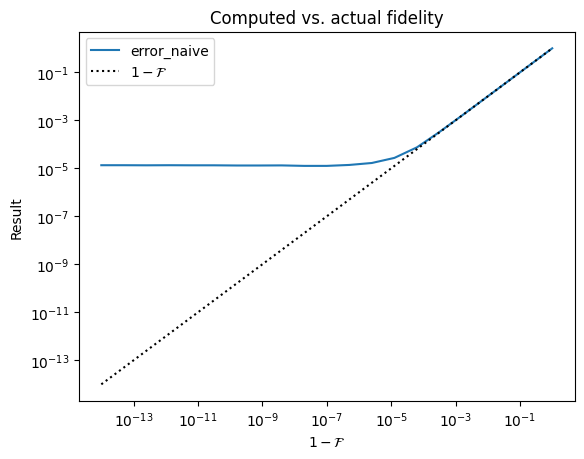
Let’s try plotting the measured fidelity vs. actual fidelity, for a range of fidelities very close to 1. (Here we plot the difference from 1, so that we can see the results easily on a log plot).

Code

import numpy as np
from matplotlib import pyplot as plt

def generate_random_complex_unit_vector(dimension):
    rtn = np.zeros((dimension,), dtype=np.complex64)
    rtn += np.random.standard_normal(dimension)
    rtn += 1j * np.random.standard_normal(dimension)
    rtn /= np.linalg.norm(rtn)
    return rtn

def generate_random_orthogonal_vectors(dimension):
    a = generate_random_complex_unit_vector(dimension)
    b = generate_random_complex_unit_vector(dimension)

    # gram-schmidt, to make them orthogonal
    b -= np.vdot(a, b) * a
    b /= np.linalg.norm(b)

    return a, b

def plot_fidelity_measure(dimension, x_min, x_max, n_pts, fidelity_funcs):
    a, b = generate_random_orthogonal_vectors(dimension)
    
    pts = np.geomspace(x_min, x_max, n_pts)

    for fidelity_func in fidelity_funcs:
        results = []
        for target_err in pts:
            c = np.sqrt(target_err)*b + np.sqrt(1-target_err)*a
            results.append(fidelity_func(a, c))

        plt.loglog(pts, 1-np.array(results), label=r"$1 - $"+fidelity_func.__name__)
    
    plt.loglog(pts, pts, color='k', linestyle=':', label=r'$1 - \mathcal{F}$')

    plt.xlabel(r'$1-\mathcal{F}$')
    plt.ylabel('Result')

    plt.title('Computed vs. actual fidelity')

    plt.legend()

plot_fidelity_measure(
    dimension=2**20, 
    x_min=1E-14, 
    x_max=1, 
    n_pts=21, 
    fidelity_funcs=[fidelity_naive]
)

The reason for the discrepancy is that in the inner product, we are summing values \(a_i^* b_i\) that have magnitude \(\mathcal{O}(1/d)\), but the “important part” of each term (that prevents the sum from being exactly 1) is of order \(\mathcal{O}(\epsilon/d)\), where \(\epsilon = 1-\mathcal{F}\). If \(\epsilon\) is very small, this “content” will be lost to floating point errors. Instead, we’d like to figure out a way to sum that content we care about directly.

Consider the following fact: \[ |\ket{a}-\ket{b}|^2 = 2 - 2\mathrm{Re}\left[ \braket{a | b} \right] \] So, the square of the norm of the difference gives the ~vibes~ of \(1 - \left|\braket{a|b}\right|\), except it cares about the relative phase between \(\ket{a}\) and \(\ket{b}\). The upshot is that it should be numerically stable to compute, because the elements of the difference vector will be of order \(\mathcal{O}(\epsilon/d)\). The key idea is that we can use it to measure \(|\braket{a|b}|\) if we ensure there is no relative phase between \(\ket{a}\) and \(\ket{b}\).

Let \(c = \braket{a|b}/|\braket{a|b}|\). Then by construction \(\braket{c a | b} = |\braket{a | b}| = \mathrm{Re}\left[ \braket{c a | b} \right]\). Combining this with the above, we may define \(e = |c \ket{a}-\ket{b}|^2\) and then: \[ |\braket{a | b}| = 1 - e/2 \] and thus \[ \mathcal{F} = |\braket{a|b}|^2 = (1 - e/2)^2 \] or, if we’re interested in the difference from 1, \[ 1-\mathcal{F} = e - e^2/4 \] This is an exact expression (we didn’t use any approximations to get it), but it also will not suffer from numerical instability for values close to zero.

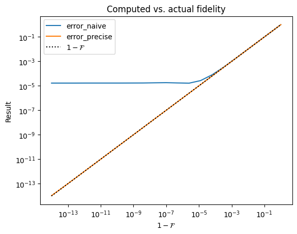
Pretty cool! Let’s try it:

def fidelity_precise(a, b):
    inner_prod = np.vdot(a, b)

    # to avoid division by zero
    if inner_prod == 0:
        return 0.0
        
    c = inner_prod / np.abs(inner_prod)
    diff = c*a - b
    e = np.real(np.vdot(diff, diff))  # imag part is zero
    return (1-e/2)**2

Code

plot_fidelity_measure(
    dimension=2**20, 
    x_min=1E-14, 
    x_max=1, 
    n_pts=21, 
    fidelity_funcs=[fidelity_naive, fidelity_precise]
)

It works super well! Yay!