Chapter 6 Implementing interactive protocols on a trapped-ion quantum computer
6.1 Introduction
To date, the field of experimental quantum computation has largely operated in a non-interactive paradigm, where classical data is extracted from the computation only at the very last step. While this has led to many exciting advances, it has also become clear that in practice, interactivity—made possible by mid-circuit measurements performed on the quantum device—will be crucial to the operation of useful quantum computers. For example, within quantum error correction, projective mid-circuit measurements are used to convert a continuum of possible errors into a specific discrete set of errors which can be corrected, as has been demonstrated in a recent experiment [NC11, RBL+21]. Certain quantum machine learning algorithms also leverage mid-circuit measurements to introduce essential non-linearities [CCL19]. Recent work has shown that interaction can do much more: it has emerged as an indispensable tool for verifying the behavior of untrusted quantum devices [MAH18, BCM+21, GV19], and even for testing the fundamentals of quantum mechanics itself [ABE+17].
Consider the scenario of a classical computer sending commands to an untrusted quantum device that it cannot feasibly simulate. This could consist of a lab computer testing a new, large quantum device, but also perhaps a user connecting to a quantum cloud computing service over the internet. At first sight, the inability of the classical machine to simulate the quantum one seems to pose a difficulty for certifying the output. This challenge mirrors one explored in the field of classical computer science, which asks whether a skeptical, computationally-bounded “verifier,” who is not powerful enough to validate a given statement on their own, can be convinced of its veracity by a more powerful but untrusted “prover.” Several decades ago, this idea began to be pursued through a novel tool called an interactive proof. In these protocols, the verifier’s goal is to accept only valid statements, regardless of whether the prover behaves honestly or attempts to cheat. One of the greatest achievements of computational complexity theory is a set of results showing that in certain scenarios multiple rounds of interaction allow the verifier to detect cheating by even arbitrarily computationally powerful provers [GMR89, LFK+90, SHA92]. The essential idea is that interaction can force the prover to commit to some piece of information early in the protocol, upon which the verifier follows up with queries that can only be answered consistently if the prover is being truthful. In exciting recent developments, success has been found in the application of this idea to quantum computing: interactive proofs have been shown to allow the verification of a number of practical quantum tasks, including random number generation, [BCM+21] remote quantum state preparation, [GV19] and the delegation of computations to an untrusted quantum server.[MAH18] Perhaps the most direct application of an interactive protocol is for a “cryptographic proof of quantumness”—a protocol that allows a quantum device to convincingly demonstrate its non-classical behavior to a polynomial-time classical verifier, by performing a task that is assumed to be computationally hard for a classical machine yet is efficient to check [BCM+21, BKV+20, KCV+22].
The simplest proof of quantumness in general is a Bell test (which does not rely on a computational hardness assumption) [BEL64]. It uses entanglement to generate correlations that would be impossible to classically reproduce without communication. While the Bell test’s simplicity is attractive, avoiding the communication loophole requires the use of multiple quantum devices which are separated by considerable distance. [HBD+15, SMC+15, GVW+15] In order to prove the quantumness of a single “black-box” quantum device whose inner workings are hidden from the verifier, one can instead rely on differences in classical and quantum computational power—in other words, asking the device to demonstrate quantum computational advantage. In contrast to recent sampling-based tests of quantum computational advantage [AAB+19, ZWD+20, WBC+21, ZCC+22, AA11, LBR17, HM17, BIS+18, BFN+19, AG20], in a cryptographic proof of quantumness the verification step must also be efficient. While in principle any algorithm that exhibits a quantum speedup and has an efficiently-verifiable output could be used for this purpose, most such experiments are infeasible today because the necessary circuits are far too large to run successfully on current quantum computers. Remarkably, it has been shown that interactive proofs provide a way to reduce the experimental cost (in qubits and gate depth) of this type of test, while maintaining efficient verification and classical hardness.
In practice, the experimental implementation of interactivity is extremely challenging. It requires the ability to independently measure subsets of qubits in the middle of a quantum circuit and to continue coherent evolution afterwards. Unfortunately, the measurement of a target qubit typically disturbs neighboring qubits, degrading the quality of computations following the mid-circuit measurement. One solution, which finds commonality among atomic quantum computing platforms, is to spatially isolate target qubits via shuttling [HEN21, BLS+22, PDF+21]. While daunting from the perspective of quantum control, experimental progress toward coherent qubit shuttling opens the door not only to interactivity but also to distinct information processing architectures [KMW02].
In this work, we implement two complementary interactive cryptographic proof of quantumness protocols, shown in the schematic of Fig. 6.1, on an ion trap quantum computer with up to 11 qubits using circuits with up to 145 gates. The interactions between verifier and prover are enabled by the experimental realization of mid-circuit measurements on a portion of the qubits (Fig. 6.2) [RBL+21, PDF+21, WKE+19]. The first protocol involves two rounds of interaction and is based upon the learning with errors (LWE) problem [REG09, REG10]. The LWE construction is unique because it exhibits a property known as the “adaptive hardcore bit” [BCM+21] (described in more detail in the next section), which enables a particularly simple measurement scheme. The second protocol is the one introduced in Chapter 5, which circumvents the need for this special property and thus applies to a more general class of cryptographic functions. By using an additional round of interaction, the cryptographic information is condensed onto the state of a single qubit. This makes it possible to implement a cryptographic proof of quantumness which is as hard to spoof classically as factoring, but whose associated circuits can exhibit an asymptotic scaling much simpler than Shor’s algorithm ( instead of , in terms of gate counts)[KCV+22].
6.2 Trapdoor claw-free functions
Both interactive protocols (Fig. 6.1) rely upon a cryptographic primitive called a trapdoor claw-free function (TCF) [GMR84]—a 2-to-1 function for which it is cryptographically hard to find two inputs mapping to the same output. Such pairs of colliding inputs are called “claws”, and the term “claw-free” refers to the hardness of finding them. The function also has a “trapdoor,” a secret key with which it is easy to compute the inputs and from any output . The intuition behind the protocols is the following: Despite the claw-free property, a quantum computer can efficiently generate a superposition of two inputs that form a claw; this is most simply realized by evaluating on a superposition of the entire domain, and then collapsing to a single output, , via measurement. In this way, a quantum prover can generate the state , where is the measurement result. The prover now sends to the verifier, who then uses the trapdoor to compute and , thus giving the verifier full knowledge of the prover’s quantum state. The verifier then asks the prover to measure . In particular, they request either a standard basis measurement (yielding or in full), or a measurement that interferes the states and . (Note that the value of , and by association and , changes each time the protocol is executed, so it is not possible to find a collision by simply repeating this process with a standard basis measurement multiple times). The verifier checks the measurement result on a per-shot basis. Crucially, consistently producing correct values for these measurements results is impossible for a classical prover (assuming they cannot find a claw of the TCF), so reliably returning correct results constitutes a proof of quantumness.
6.2.1 The learning with errors problem
It is believed to be classically intractable to recover an input vector from the result of certain noisy matrix-vector multiplications—this constitutes the LWE problem [REG09, REG10]. In particular, a secret vector, , can be encoded into an output vector, , where is a matrix and is an error vector corresponding to the noise. Using the LWE problem, a TCF can be constructed as , where is a single bit that controls whether gets added to and denotes a rounding operation [BPR12, AKP+13] (see Methods section 6.6.7 for additional details). Here, and play the role of the trapdoor, and a claw corresponds to colliding inputs with and . By implementing the protocol described above and illustrated in Figure 6.1, the prover is able to generate the state . For the aforementioned “interference” measurement, the prover simply measures each qubit of the superposition in the basis. Crucially, the result of this measurement is cryptographically protected by the adaptive hardcore bit property, which is a strengthening of the claw-free property [BCM+21]. Informally, it says that for any input (of the prover’s choosing), it is cryptographically hard to determine even a single bit of information about (as opposed to the entire value, which is the guarantee of the claw-free assumption).
6.2.2 Rabin’s function
The function , with being the product of two primes, was originally introduced in the context of digital signatures [RAB79, GMR88]. This function has the property that finding two colliding inputs (a claw) in the range is as hard as factoring . Moreover, the prime decomposition can serve as a trapdoor, enabling one to invert the function for any output. Thus, is a trapdoor claw-free function. However, does not have the adaptive hardcore bit property, making the simple -basis “interference” measurement (described in the LWE context above) not provably secure. To get around this, we perform the “interference” measurement differently. First, the verifier chooses a random subset of the qubits of the superposition, and the prover stores the parity of that subset on an ancilla. Then, the prover measures everything except the ancilla in the basis. Given our cryptographic assumption that the prover cannot find a claw, the prover cannot guess the polarization of the remaining ancillary qubit. This is directly analogous to how, in Bell experiments, the assumption of no-signaling-faster-than-light implies that if Alice measures one half of an EPR pair, a space-like separated Bob who holds the other half is unable to immediately guess its polarization. Following this intuition, the verifier requests a measurement of the ancilla qubit in the or basis, effectively completing the Bell test [BEL64, CHS+69]; the verifier accepts if the prover returns the more likely measurement outcome. Crucially, the dependence of the measurement result on the claw renders it infeasible to guess classically [KCV+22].
6.3 Implementing an interactive cryptographic proof
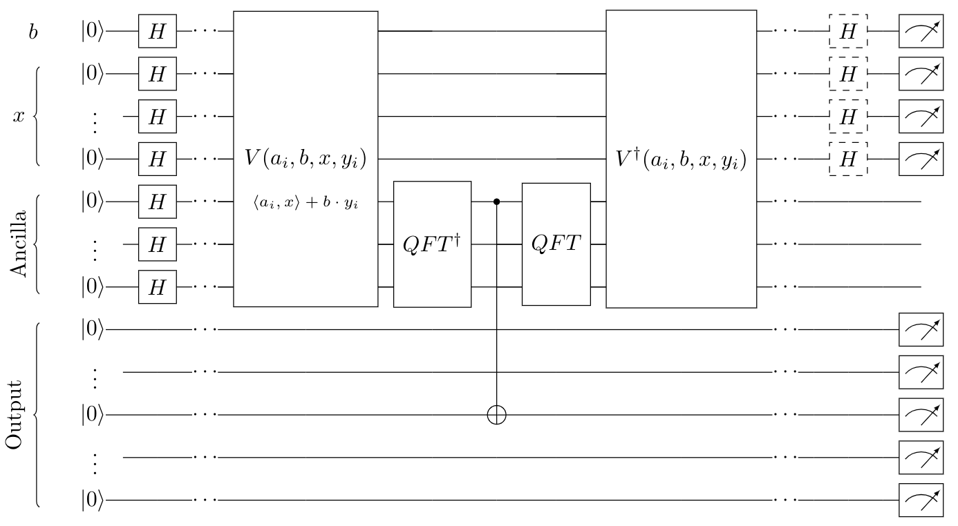
In order to implement an interactive cryptographic proof of quantumness, we design quantum circuits for both the LWE- and factoring-based protocols. The high-level circuit diagrams are shown in Figs. 6.3(a,b). In both cases, the circuits are composed of several sections. First, the prover creates a uniform superposition via Hadamard gates, where is the number of input qubits. Then, they compute the TCF on an output register using this superposition as input [Fig. 6.3(a,d)], thereby generating the state . Next, the prover performs a mid-circuit measurement on the output register, collapsing the state to . Finally, based on the verifier’s choice of measurement scheme (i.e. standard vs. interference), the prover must perform additional coherent gates and measurements (see Methods for a full description of the quantum circuits used).
We implement both interactive protocols using an ion trap quantum computer, with a base chain length of 15 ions (Fig. 6.2); for each 171Yb+ ion, a qubit is encoded in a pair of hyperfine levels [MCD+21]. The quantum circuits are implemented via the consecutive application of native single and two-qubit gates using individual optical addressing [Fig. 6.2(a)] [EDN+21]. In order to realize rapid successive two-qubit interactions, we position the ions in a single, closely-spaced linear chain [Fig. 6.2(d)].
This geometry makes it challenging to implement mid-circuit measurements, because light scattered from nearby ions during a state-dependent fluorescence measurement can destroy the state of the other ions. To overcome this issue, we vary the voltages on the trap electrodes to split and shuttle the ion chain, thereby spatially isolating the ions not being measured (Fig. 6.2a-c). Depending on the protocol, the ion chain is split into either two or three segments. To measure the ions in a particular segment, we re-shape the electric potential to align the target segment with the detection system. In addition, we calibrate and correct for spatial drifts of the optical beams, variations of stray fields, and unwanted phase accumulation during shuttling (see Methods sections 6.6.2, 6.6.5 for additional details).
In this demonstration, the qubits play the role of the prover and the classical control system plays the role of the verifier. This allows us to compile the decisions of the verifier into the classical controller prior to execution of the quantum circuit.
6.4 Beating the classical threshold
As in a Bell test, even a classical prover can pass the verifier’s challenges with finite probability. If the classical prover cannot find a claw in the TCF (which is assumed to be the case for sufficiently large problem sizes), this probability can be bounded by an asymptotic “classical threshold”—which a quantum prover must exceed to demonstrate advantage. (For a discussion of what it means that this threshold is “asymptotic” rather than absolute, see the Methods section 6.6.9). For both protocols, this threshold is best expressed in terms of the probabilities of passing the verifier’s “standard basis” and “interference” checks, which we denote as and , respectively (see Methods section 6.6.3 for the definition of the verifier’s checks). For the LWE-based protocol, the classical threshold is given by (derivation in Methods section 6.6.10); for the factoring-based protocol, it is given by . [KCV+22] In both cases, is a function which goes to zero exponentially in the problem size. An intuition for the difference between the thresholds is that the factoring-based protocol requires an additional round of interaction during the “interference” test.
As depicted in Figure 6.3(b), we perform multiple instances of the LWE-based protocol for different matrices and noise vectors . For each of the verifier’s possible choices, we repeat the experiment times to collect statistics. This yields the experimental probabilities and , allowing us to confirm that the quantum prover exceeds the asymptotic classical threshold in all cases. The statistical significance by which the bound is exceeded (more than in all cases, see Table 6.2 in the Methods section 6.6.1) is shown in Figure 3(b). Figure 6.3(e) depicts the analogous results for the factoring-based protocol, where the different instances correspond to different values of . For all but , which requires the deepest circuit, the results exceed the asymptotic classical bound with more than statistical significance. We utilize an error-mitigation strategy based on excluding iterations where is measured to be invalid, i.e. not in the range of (see 6.6.4); effectively, this implements a post-selection which suppresses bit-flip errors [KCV+22].
To further analyze the performance of each branch of the interactive protocol, corresponding to the verifier’s choices [Figs. 6.3(c,f)], we define the relative performance for each branch, where is the probability that an error-free quantum prover would pass, is the probability that a random guesser would pass, and is the passing rate measured in the experiment. This criterion is a way of isolating and evaluating the effect of noise on the success probabilities of each branch, by removing effects such as the fact that an error-free run may still happen to get rejected by the verifier, which is inherent to the protocol. In particular, for a perfect (noise-free) quantum prover always, and for a device so noisy that its outputs are uniformly random . To probe the noise effects of the mid-circuit measurements, we implement two versions of the protocols: one interactively (the normal protocol) and another with all measurements delayed until the end of the circuit, and compare the relative performance between the two cases. We emphasize that the delayed-measurement version is only a tool to probe our experimental system, and may be vulnerable to classical spoofing even if it were run at large problem sizes where the other cryptographic assumptions hold—the interaction enabled by mid-circuit measurements is crucial.
For the LWE-based protocol, there are two rounds of interaction, corresponding to the two branches, I and II shown in Fig. 6.3(c), while for the factoring-based protocol there are three rounds of interaction [Fig. 6.3(f)]. By comparing the relative performance between the interactive and delayed-measurement versions of our experiment, we are able to probe a subtle feature of the protocols—namely, that certain branches are robust to additional decoherence induced by the mid-circuit measurements. Microscopically, this robustness arises because these branches (thick lines, Figs. 6.3c,f) do not depend on the phase coherence between and . In particular, this is true for the standard-basis measurement branches in both protocols, and also for the branches of the factoring-based protocol where the ancilla is polarized in the basis (see Methods section 6.6.6). Noting that mid-circuit measurements are expected to induce mainly phase errors, one would predict that those branches insensitive to phase errors should yield similar performance in both the interactive and delayed-measurement cases. This is indeed borne out by the data.
6.5 Discussion and outlook
There are two main experimental challenges to demonstrating quantum computational advantage via interactive protocols: 1) integrating mid-circuit measurements into arbitrary quantum circuits, with sufficiently high overall fidelity to pass the verifier’s tests, and 2) scaling the protocols up to large enough problem sizes that it is classically infeasible to break the cryptographic assumptions. In this work we have overcome the first obstacle, successfully implementing two interactive cryptographic proofs of quantumness with high enough fidelity to pass the verifier’s challenges. We leave the second challenge, of scaling these protocols up, to a future work. We estimate that one should be able to perform a cryptographic proof of quantum computational advantage using qubits (see Methods section 6.6.13). Note that while this qubit count is comparable to some implementations of Shor’s algorithm, the circuits are orders of magnitude smaller in gate count ( vs. ) and depth [KCV+22]. Even with those smaller circuits, the challenge on near-term devices will almost certainly remain the circuit depth; interestingly, recent advances suggest that our interactive protocols can be performed in constant depth at the cost of a larger number of qubits [HL21, LG22]. Once this scaling is achieved in an experiment, it will demonstrate directly-verifiable quantum computational advantage. This would mark a new step forward from recent sampling experiments, which have demonstrated the system sizes and fidelities necessary to make classical simulation extremely hard or impossible [AAB+19, ZWD+20, WBC+21, ZCC+22, AA11, LBR17, HM17, BIS+18, BFN+19, AG20] but have no method to directly and efficiently verify the output (and moreover, practical strategies for a classical impostor to replicate the sampling are still being explored [HZN+20, PZ22, GK21, PCZ22, LLL+21c, LGL+21a, GKC+21, AGL+23]).
Our work also opens the door to a number of other intriguing directions. A clear next step is to apply the power of quantum interactive protocols to achieve more than just quantum advantage—for example, pursuing such tasks as certifiable random number generation, remote state preparation and the verification of arbitrary quantum computations [BCM+21, GV19, MAH18]. We emphasize that unlike e.g. Bell-test based protocols for random number generation, interactive proofs allow us to perform these cryptographic tasks with a single “black-box” prover with which the verifier can only interact classically. This has the potential to allow these types of protocols (including our cryptographic proofs of quantumness) to be performed on a remote prover, such as a quantum cloud service on the internet, enabling a wide variety of practical applications. Finally, the advent of mid-circuit measurement capabilities in a number of platforms [PDF+21, WKE+19, CTI+21, RRG+22], enables the exploration of new phenomena such as entanglement phase transitions [SRN19, LCF18, NNZ+22] as well as the demonstration of coherent feedback protocols including quantum error correction [RBL+21].
6.6 Additional proofs and data
6.6.1 Result data
In Tables 6.1 and 6.2 we present the numerical results for each configuration of the experiment, along with the number of samples obtained ( and ), the measure of quantumness , and the statistical significance of the result (see Methods Section 6.6.11 for a description of how the significance is calculated).
We note that for the computational Bell test protocol, the sample size is less than the actual number of shots that passed postselection (ultimately leading to slightly less statistical significance than might otherwise be expected). This is because the sample size varied for different values of the verifier’s string , yet we are interested in the passing rate averaged uniformly over all (not weighted by number of shots). To account for this, we simply took the -value with the fewest number of shots, and computed as if every value had had that sample size (even if some values of had more).
We also note that in some cases the statistical significance denoted here may be higher than that visually displayed in Figure 6.3 of the main text; this is because the contour lines in that figure correspond to the configuration with the smallest sample size.
| N |
|
Quantumness | Significance | ||||||
|---|---|---|---|---|---|---|---|---|---|
| 8 | interactive | 0.952 | 0.777 | 4096 | 15267 | 0.061 | |||
| 8 | delayed | 0.985 | 0.837 | 2736 | 17361 | 0.334 | |||
| 15 | delayed | 0.934 | 0.798 | 2361 | 31353 | 0.127 | |||
| 16 | delayed | 0.927 | 0.790 | 3874 | 53550 | 0.087 | |||
| 21 | delayed | 0.864 | 0.700 | 2066 | 27944 | -0.338 | — |
| Instance |
|
Quantumness | Significance | ||||||
|---|---|---|---|---|---|---|---|---|---|
| 0 | interactive | 0.757 | 0.710 | 8000 | 13381 | 0.178 | |||
| 0 | delayed | 0.793 | 0.880 | 10000 | 9415 | 0.553 | |||
| 1 | interactive | 0.601 | 0.737 | 8000 | 7622 | 0.075 | |||
| 1 | delayed | 0.608 | 0.803 | 8000 | 7547 | 0.215 | |||
| 2 | interactive | 0.720 | 0.704 | 14000 | 15310 | 0.129 | |||
| 2 | delayed | 0.730 | 0.839 | 4000 | 3735 | 0.409 | |||
| 3 | interactive | 0.740 | 0.704 | 8000 | 15189 | 0.148 | |||
| 3 | delayed | 0.730 | 0.772 | 8000 | 7528 | 0.274 |
6.6.2 Trapped ion quantum computer
The trapped ion quantum computer used for this study was designed, built, and operated at the University of Maryland and is described elsewhere [EDN+21, CEN+22]. The system consists of a chain of fifteen single 171Yb+ ions confined in a Paul trap and laser cooled close to their motional ground state. Each ion provides one physical qubit in the form of a pair of states in the hyperfine-split ground level with an energy difference of 12.642821 GHz, which is insensitive to magnetic fields to first order. The qubits are collectively initialized through optical pumping, and state readout is accomplished by state-dependent fluorescence detection [OYM+07]. Qubit operations are realized via pairs of Raman beams, derived from a single 355-nm mode-locked laser [DLF+16]. These optical controllers consist of an array of individual addressing beams and a counter-propagating global beam that illuminates the entire chain. Single qubit gates are realized by driving resonant Rabi rotations of defined phase, amplitude, and duration. Single-qubit rotations about the z-axis, are performed classically with negligible error. Two-qubit gates are achieved by illuminating two selected ions with beat-note frequencies near motional sidebands and creating an effective Ising spin-spin interaction via transient entanglement between the two ion qubits and all modes of motion [MS99, SdZ99, MSJ00]. To ensure that the motion is disentangled from the qubit states at the end of the interaction, we used a pulse shaping scheme by modulating the amplitude of the global beam [CDM+14].
6.6.3 Verifier’s checks
In this section we explicitly state the checks performed by the verifier to decide whether to accept or reject the prover’s responses for each run of the protocol. We emphasize that these checks are performed on a per-shot basis, and the empirical success rates and are defined as the fraction of runs (after postselection, see below) for which the verifier accepted the prover’s responses.
For both protocols, the “A" or “standard basis" branch check is simple. The prover has already supplied the verifier with the output value ; for this test the prover is expected to measure a value such that . Thus in this case the verifier simply evaluates for the prover’s supplied input and confirms that it is equal to .
For the “B" or “interference" measurement, the measurement scheme and verification check is different for the two protocols. For the LWE-based protocol, the interference measurement is an -basis measurement of all of the qubits holding the input superposition . This measurement will return a bitstring of the same length as the number of qubits in that superposition, where for each qubit, the corresponding bit of is 0 if the measurement returned the eigenstate and 1 if the measurement returned the eigenstate. The verifier has previously received the value from the prover and used the trapdoor to compute and ; the verifier accepts the string if it satisfies the equation
| (6.1) |
where denotes the binary inner product, i.e. . It can be shown that a perfect (noise-free) measurement of the superposition will yield a string satisfying Eq. 6.1 with probability 1.
The interference measurement for the computational Bell test involves a sequence of two measurements (in addition to the first measurement of the string ). The first measurement yields a bitstring as above. After performing that measurement, the prover holds the single-qubit state , where is the binary inner product as above and is a random bitstring supplied by the verifier. This state is one of , and is fully known to the verifier after receiving (via use of the trapdoor to compute and ). The second measurement is of this single qubit, in an intermediate basis or chosen by the verifier. For any of the four possible states, one eigenstate of the measurement basis will be measured with probability (with the other having probability ), just as in a Bell test. The verifier accepts the measurement result if it corresponds to this more-likely result; an ideal (noise-free) prover will be accepted with probability (see Figure 6.3 of the main text).
6.6.4 Post-selection
Both the factoring-based and LWE-based protocols involve post-selection on the measurement results throughout the experiment.
| Instance | Delayed Measurement | Interactive Measurement |
| 0 | 3753/4000 | 13381/14000 |
| 1 | 7547/8000 | 7622/8000 |
| 2 | 3735/4000 | 15310/16000 |
| 3 | 7528/8000 | 15144/16000 |
| N | Interactive | Branch | Runs kept/Total |
| 8 | Yes | A | 4096/9000 |
| 8 | Yes | B, r=01 | 5093/12000 |
| 8 | Yes | B, r=10 | 5089/12000 |
| 8 | Yes | B, r=11 | 5492/12000 |
| 8 | No | A | 2736/6000 |
| 8 | No | B, r=01 | 5787/12000 |
| 8 | No | B, r=10 | 5818/12000 |
| 8 | No | B, r=11 | 5865/12000 |
| 15 | No | A | 2361/6000 |
| 15 | No | B, r=001 | 4636/12000 |
| 15 | No | B, r=010 | 4532/12000 |
| 15 | No | B, r=011 | 4666/12000 |
| 15 | No | B, r=100 | 4496/12000 |
| 15 | No | B, r=101 | 4727/12000 |
| 15 | No | B, r=110 | 4479/12000 |
| 15 | No | B, r=111 | 4673/12000 |
| N | Interactive | Branch | Runs kept/Total |
| 16 | No | A | 3874/6000 |
| 16 | No | B, r=001 | 7842/12000 |
| 16 | No | B, r=010 | 7847/12000 |
| 16 | No | B, r=011 | 7732/12000 |
| 16 | No | B, r=100 | 7936/12000 |
| 16 | No | B, r=101 | 7870/12000 |
| 16 | No | B, r=110 | 7841/12000 |
| 16 | No | B, r=111 | 7650/12000 |
| 21 | No | A | 2066/6000 |
| 21 | No | B, r=001 | 3992/12000 |
| 21 | No | B, r=010 | 4273/12000 |
| 21 | No | B, r=011 | 4137/12000 |
| 21 | No | B, r=100 | 4182/12000 |
| 21 | No | B, r=101 | 4193/12000 |
| 21 | No | B, r=110 | 4261/12000 |
| 21 | No | B, r=111 | 4221/12000 |
For the factoring-based protocol, this post-selection is performed on the measured value of the output register . Due to quantum errors in the experiment, in practice it is possible to measure a value of that does not correspond to any inputs of the TCF—that is, there do not exist for which , due to noise. Because such a result would not be possible without errors, measuring such a value indicates that a quantum error has occurred [KCV+22]. Thus, we perform post-selection by discarding all runs for which the measured value does not have two corresponding inputs.
On the other hand, for the LWE protocol, we post-select in order to satisfy the conditions for the adaptive hardcore bit property to hold, as without this property, the protocol could be susceptible to attacks. In particular, the adaptive hardcore bit property requires that the result obtained from measuring the register using the “interference” measurement scheme be a nonzero bitstring [BCM+21]. Hence, we simply post-select on this condition for the LWE case. Tables 6.3 and 6.4 explicitly show how many runs are kept using each post selection scheme.
We note that in both cases, post-selection does not affect the soundness of the protocols. We only require that a non-negligible fraction of runs pass post-selection (to give good statistical significance for the results). This is indeed the case for our experiment, as can be seen in Tables 6.3, 6.4, as well as the statistical significance of the results in Tables 6.1, 6.2.
6.6.5 Shuttling and mid-circuit measurements
We control the position of the ions and run the split and shuttling sequences by changing the electrostatic trapping potential in a microfabricated chip trap [MAU16] maintained at room temperature. We generate 40 time-dependent signals using a multi-channel DAC voltage source, which controls the voltages of the 38 inner electrodes at the center of the chip and the voltages of two additional outer electrodes. Owing to the strong radial confining potential used (with secular trapping frequencies near MHz), the central electrodes’ potential affects predominantly the axial trapping potential, and in turn, generates movement predominantly along the linear trap axis. To maintain the ions at a constant height above the trap surface, we simulate the electric field based on the model in Ref. [MAU16], and compensate for the average variation of its perpendicular component by controlling the voltages of the outer two electrodes.
In the first sequence, we split the 15-ion chain into two sub-chains of 7 and 8 ions, and shuttle the 8-ion group to mm away from the trap center at . We then align the 7-ion chain with the individual-addressing Raman beams for the first mid-circuit measurement. For the LWE-based protocol, we then reverse the shuttling process and re-merge the ions to a 15-ion chain, completing the circuit and performing a final measurement. For the factoring-based protocol, we shuttle the 8-ion sub-chain to the trap center and the 7-ion sub-chain to mm. We then split this chain into 5- and 3-ion sub-chains, shuttle the 3-ion sub-chain to mm, and align the 5 ions at the trap center with the Raman beams to perform additional gates and a second mid-circuit measurement. Finally, we move away the measured ions and align the 3-ion group to the center of the trap to complete the protocol. Reversing the sequence then prepares the ions in their initial state. For each protocol, all branches use the same shuttling sequences but differ in the qubit assignment and the realized gates. The mid-circuit measurement duration was experimentally determined prior to the experiment by maximizing the average fidelity of a Ramsey experiment using single-qubit gates, approximately optimizing for the trade-off between efficient detection of each sub-chain and stray light decoherence.
To enable efficient performance of the split and shuttling sequences we numerically simulate the electrostatic potential and the motional modes of the ions that are realized in the sequences. We minimize heating of the axial motion from low-frequency electric-field noise by ensuring that the calculated lowest axial frequency does not go below KHz. We also minimize the frequency of ions loss due to collisions with background gas by maintaining a calculated trap depth of at least meV for each of the sub-chains throughout the shuttling sequences. The simulations enable efficient alignment of the sub chains with the Raman beams, taking into account the variation of the potential induced by all electrodes.
We account and correct for various systematic effects and drifts which appear in the experiment. To eliminate the effect of systematic variation of the optical phases between the individual beams on the ions, we align each ion with the same individual beam throughout the protocol. Prior to the experiment, we run several calibration protocols which estimate the electrostatic potential at the center of the trap through a Taylor series representation up to the fourth order, estimating the dominant effect of stray electric fields on the precalculated potential. We then cancel the effect of these fields using the central electrodes during the alignment and split sequences, as these sequences are most sensitive to the exact shape of the actual electrostatic potential. Additionally, we routinely measure the common-mode drift of the individual addressing optical Raman beams along the linear axis of the trap and correct for them by automatic repositioning of the ions achieved by varying the potential.
During shuttling, the ions traverse an inhomogeneous magnetic field and consequently, each ion spin acquires a shuttling-induced phase which depends on its realized trajectory. We calibrate this by performing a Ramsey sequence in which each qubit is put in a superposition of before shuttling, and after the shuttling gates are applied, with scanned from to . Fitting the observed fringe for each ion enables estimation of the phases , which are corrected in the protocols by application of the inverse operation after shuttling.
6.6.6 Circuit construction of the factoring-based protocol
In this section, we describe the procedure for preparing the quantum superposition of all the claws in the factoring-based protocol, as shown in Fig. 6.3(a) of the main text.
This is achieved by generating
| (6.2) |
and then measuring the register. We calculate using a unitary to encode the function into the phase of the register and applying a inverse quantum Fourier transform (QFT†) to extract the result.
To start, we apply Hadamard gates to all qubits to prepare a uniform superposition of all the possible bit strings for the and registers:
| (6.3) |
where is the normalization factor.
Next, we evolve the state with the unitary . Since the phase has period , the unitary is equivalent to . We now show how to efficiently implement on the ion trap quantum computer.
First, note the multiplication in the phase can be expressed as a sum of bit-wise multiplication
| (6.4) |
This bit-wise multiplication can be expressed using Pauli operators:
| (6.5) |
We then organize the operators into three terms:
| (6.6) |
We use ’s, ’s, and ’s to represent the phases generated by these terms, which can be calculated from Eq. 6.5. The third term contains single-qubit rotations that are implemented efficiently as software-phase advances. The interactions in the second term are implemented as gates sandwiched between single qubit rotations. The first term includes three-body interactions, which can be decomposed using interactions using the following relation:
| (6.7) |
This decomposition enables efficient construction of the following cascade of interactions:
| (6.8) |
| (6.9) |
which are efficiently implemented using the native interaction and single-qubit rotations.
Using the decomposition above, we can implement the first term in Eq. 6.6 using the circuit shown in Fig. 6.4.
With this term implemented, we complete the construction of the full unitary . After applying the unitary, we obtain the state
| (6.10) |
We then apply the inverse quantum Fourier transform to the register, which gives us:
| (6.11) |
Next, we measure the register to find an output , and the -register contains the superposition of a colliding input pair.
The number of qubits used to represent in experiments are 3, 4, 4, and 5 for , , , and , respectively. The number of qubits used to represent in experiments equals the length of the string in Table 6.4.
6.6.7 Circuit construction of the LWE-based protocol
In this section, we describe the procedure for implementing the circuit , displayed in Fig. 6.3(d). Here, the matrix and vector are classical inputs, and the bit and vector are quantum values held in the qubits to which the unitary is applied. The circuits evaluate the function in superposition, where denotes a rounding operation corresponding to taking the most significant bit of each component in the vector . (It should be noted that this specific function, which uses rounding, differs from the TCF used by Brakerski et al. [BCM+21], but is nevertheless still a TCF [LG22].) This TCF is based on the LWE problem: for a secret vector and “noise” vector , find (or equivalently ) with knowledge of only and . The LWE assumption states that doing so is cryptographically hard. It is straightforward to see that finding claws in the function is as hard as breaking the LWE assumption, by observing that for a colliding pair , (up to the noise vector , whose effect disappears due to the rounding).
In our implementation, the matrix and vector are sampled uniformly at random by the verifier11 1 Technically, the matrix is sampled together with the TCF trapdoor. However, as explained in [BCM+21], the distribution from which the matrix is sampled is statistically close to a uniform distribution over . The vector is sampled from a discrete Gaussian distribution (see Brakerski et al. [BCM+21] for more details on the parameter choices). The verifier constructs and sends and to the prover.
To perform the coherent evaluation, the prover will use three registers (for the and inputs, as well as for the output of the TCF) to create the superposition state as well as a fourth ancilla register, which will be used to perform the unitary . The prover starts by applying a layer of Hadamard gates to all input qubits and the ancilla register (that were initialized as ). The resulting state will be
| (6.12) |
for some normalization constant and where the third register is the ancilla register and the last register is the output register. In this output register, the prover must coherently add . As is an -component vector, we will explain the prover’s operations, at a high level, for each component of the vector. For the ’th component of this vector, the prover first computes the inner product modulo between the ’th row of and and places the result in the ancilla register. Since the prover has a classical description of , this will involve a series of controlled operations between the register and the ancilla register. Similar to the factoring case, this arithmetic operation is easiest to perform in the Fourier basis, which is why Hadamard gates are applied to the ancilla register. Once the inner product has been computed, the prover will perform a controlled operation between the qubit and the ancilla register in order to add the ’th component of . Finally, the prover will “copy” the most significant bit of the result into the output register. This is done via another controlled operation. The prover then uncomputes the result in the ancilla, clearing that register. In this way, the ’th component of has been added into the output register. Repeating this procedure for all components will yield the desired state
| (6.13) |
with normalization constant .
Having given the high level description, let us now discuss in more detail the specific circuits of the current implementation. From the above analysis, we can see that the total number of qubits is . In the instance for this experiment, we chose , resulting in qubits. The first register contains which requires only one qubit. In the second register, the vector consists of two components modulo , which is encoded in binary with four qubits as . The third register, the ancilla, is one modulo component and will thus consist of two qubits. Lastly, in the fourth register, we store the result of evaluating the function, which requires another four qubits. As mentioned, the matrix and the vector are specified classically. In the experiment, we considered four different input configurations, corresponding to four different choices for , and . These choices are explicitly described later in the appendix.
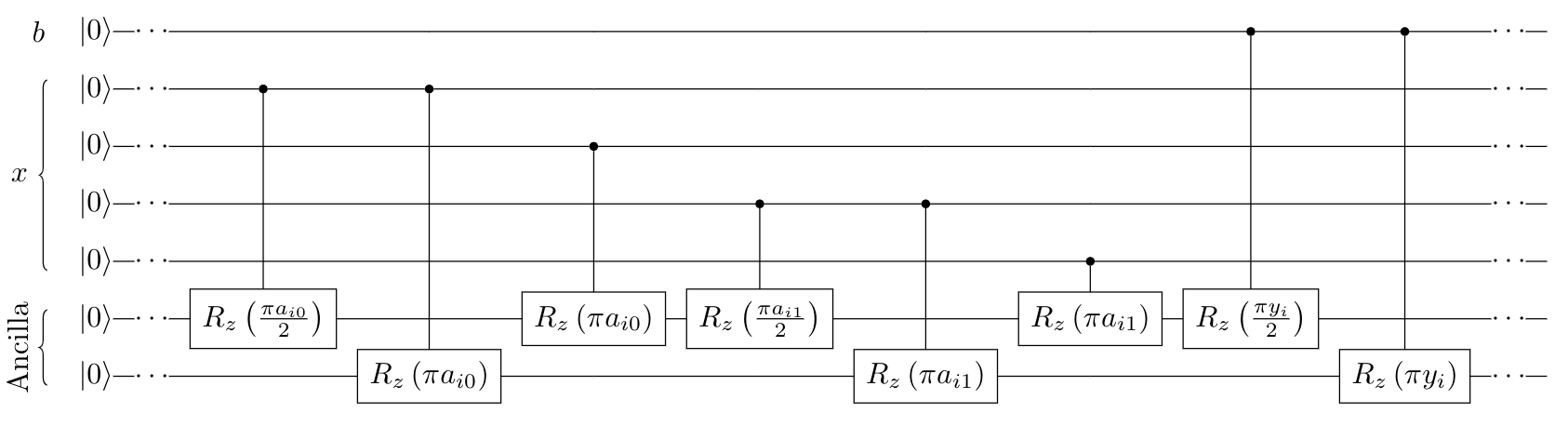
To detail the operations implemented, as discussed previously, the prover first puts the ancilla register into the Fourier basis using the quantum Fourier transform (QFT). This allows them to more easily compute in the ancilla register, where is the ’th row of the matrix and denotes the inner product modulo . The explicit rotation gates to compute this in the Fourier basis are given in Fig. 6.6. After computing this for one row , the prover converts the ancilla back into the computational basis and “copies” the most significant bit stored in the ancilla register into the output register, using a gate, to compute the rounding function. This completes the evaluation of the function for one bit. In order to reuse the qubits in the ancilla register, the prover then reverses this computation and repeats for each row of the matrix . This process of evaluating the function and reversing that computation is depicted in Fig. 6.5.
Finally, after completing the evaluation of the TCF, the prover measures the output register to recover the rounded result of for a certain value of . The prover will then measure the and registers in either the basis or basis, according to the challenge issued by the verifier. Should the verifier request measurements in the basis, the prover applies Hadamard gates on all qubits in the and registers before measuring in the computational basis.
6.6.8 Instances of LWE Implemented
| Instance | |||
| 0 | |||
| 1 | |||
| 2 | |||
| 3 |
Here, we explicitly detail the LWE instances that were used in the experiment. Recall that such an instance is defined by and , where , and for integers . In this experiment, we used for all of the instances. Table 6.5 displays the explicit matrices and vectors used.
6.6.9 Discussion of asymptotic classical threshold
In cryptography, showing that a new protocol is secure for practical use (meaning, in our case, that the proof cannot be spoofed by a classical prover) follows two broad steps: 1) proving that it is secure asymptotically (showing that the computational cost of cheating is at least superpolynomial in the problem size), and 2) picking a finite set of parameters such that cheating is not possible under certain classical resources (computational power and time, usually). What particular limitations to set on the resources available to the classical cheater is ultimately up to the user. In this section, we attempt to make precise exactly which statements are asymptotic (step 1), and how these statements make the jump in step 2 to finite, real parameters.
The first asymptotic statement, which is perhaps the most obvious, is that finding claws of the TCF is hard. In the theory papers upon which this work is based, this is shown by reducing the problem of finding claws to related problems, about which there exist standard cryptographic assumptions. [BCM+21, KCV+22] In particular, the assumptions are that the factoring and LWE problems have superpolynomial classical complexity. As discussed above, when using the test in practice we would pick finite parameters in a way that finding a claw is infeasible for the set of classical resources we wish our quantum computer to outcompete (for a rigorous demonstration of quantum advantage, probably a large supercomputer with ample runtime). Importantly, the reduction between the hardness of finding claws and breaking the cryptographic assumption is not in any sense asymptotic: for both TCFs, if a machine can find claws for a specific, finite set of parameters, they can directly use those claws to break the cryptographic assumption in practice. Therefore if the cryptographic assumption holds for a finite set of parameters, we can be sure that the claw-freeness does as well.
The second asymptotic statement that appears in the analysis of these protocols is in regard to the probability that a classical cheater passes a single iteration of the test. In Section 6.4 of the main text, we discuss the “classical thresholds,” which must be exceeded to demonstrate quantum capability. To be very precise about what we mean by this, we reproduce exactly what the theorems underlying these protocols state: if a classical prover’s true success probabilities (not the empirically determined ones, which are subject to statistical fluctuation) exceed the given bound by a non-negligible amount, that prover could be used as a subroutine in a larger program which finds a claw in the TCF in polynomial time. Thus, if it is not possible for a classical prover with certain resources to find a claw (in a TCF with some specific parameters), it is provably also not possible for a classical prover with similar resources to non-negligibly exceed the threshold. There are two asymptotic portions of this statement: the polynomial time in which the larger program extracts a claw using the prover as a subroutine (which is the reason for the word “similar” in the previous sentence), and in fact the word “negligible.” Negligible has a technical definition in cryptography, which is the sense in which we use it here. It means that a value (in this case the amount by which the threshold can be exceeded) is bounded by a function which goes exponentially to zero in the problem size. The precise form of this exponential is not intended to be determined, but instead the exponential decay is used to argue that the negligible function is “essentially” zero for any reasonable problem size that would be used in practice.
It is worth noting that for the small problem sizes we implement in this work, there is one instance in which this negligible function would meaningfully affect the classical success threshold—and we modify the protocol slightly to account for this. In the (Rabin’s function) protocol, the value sent by the verifier is supposed to be a uniformly random bitstring. If happens to be all zero, the product , whose value is supposed to be cryptographically hard to guess, is simply zero. This is not an issue for problem sizes that would be used for a full-scale test in practice, because an all-zero is extremely unlikely to occur if is of length several hundred bits. But for our smaller experiments with of only a few bits, the all-zero string represents a sizable fraction of possible . To prevent this from affecting the results, we simply choose our from the set of non-zero bitstrings rather than all bitstrings. We note that excluding the all zero string helps us better resolve the experiment’s performance, too: when the qubit measured in the last step of the protocol never interacts with any of the other qubits throughout the whole circuit, so the measurement result has nothing to do with the fidelity of the TCF circuit!
To close this discussion, it is worth taking a broader perspective and considering how the field of cryptography functions in general. Asymptotic proofs in cryptography are used to show that for any cheating machine with finite resources, the problem can always be made large enough to be hard in practice—and that the hardness grows quickly enough that this is hopefully not an unreasonable pursuit. But ultimately, the question of how large the problem needs to be is an empirical one: experts build the best possible algorithms and hardware they can to attempt to break the assumption, and then the parameters are set to be larger than the largest problem size that can be broken this way (usually with an extra buffer added to secure against improvements in the attacks). In our case, the costs of breaking both factoring and LWE have been extensively explored, and the practical parameters needed for their security against current classical computing power are well understood. As described above, because there are no asymptotic statements in the reduction from the TCF to the underlying cryptographic assumptions, these parameters can be directly used to ensure that finding claws is hard in practice. As described above, the precise relationship between the hardness of exceeding the thresholds and finding claws does rely on asymptotics, but the fact that the asymptotic function appearing in the threshold is shown to decay exponentially suggests strongly that this should not be an issue in practice.
6.6.10 Quantum-classical threshold of LWE based protocol
In this section, we state and prove the classical threshold for the LWE-based protocol. The corresponding proof for the factoring-based protocol is contained in the theory manuscript that first presented that protocol. [KCV+22]
Below, the security parameter is used in the standard cryptographic sense, as a measure of the “problem size”—it can be made larger to increase security, or smaller to improve efficiency. The specifics of how each parameter of the LWE problem is defined as a function of can be found in the definition of the LWE-based TCF, in the theory work that originally proposed it. [BCM+21]
Proposition 1.
For any classical prover, the probabilities that they pass branches A and B, and , must obey the relation
| (6.14) |
where is a negligible function of the security parameter .
Proof.
We first want to find the probability that the classical prover both responds correctly for Branch A and, for the same output that they committed to the verifier, Branch B is also correct with probability greater than , where is a non-negligible function of the security parameter . Let this second probability be denoted as
| (6.15) |
By a union bound, we arrive at a bound on the desired probability
| (6.16) |
Now, we wish to write in terms of . Let be the set of values for which . By definition, we know that with probability , the prover samples a so that they pass the verifier’s Branch B test with probability at least and at most . Similarly, we know that with probability , the prover samples a so that they pass the verifier’s Branch B test with probability at most . Hence, overall we see that the probability that the prover passes Branch B is at most the convex mixture of these two cases, i.e.
| (6.17) |
Solving for , we then obtain
| (6.18) |
Substituting this into Equation 6.16, we have
| (6.19) |
However, notice that this probability on the left hand side is the probability of breaking the adapative hardcore bit property, which we know [BCM+21] must have
| (6.20) |
where is a negligible function. Thus, combining this with Equation 6.19, we obtain the desired inequality
| (6.21) |
∎
6.6.11 Computation of statistical significance contours
Here we describe the computation of the contour lines denoting various levels of statistical significance in Figure 6.3(b,e) of the main text. Recall the probabilities and introduced in Section 6.4, which denote a prover’s probability of passing the standard basis and interference test, respectively. Assuming the cryptographic soundness of the claw-free property of the TCF, and in the limit of large problem size, any classical cheating strategy must have true values of and that obey the bound for the LWE protocol and for the factoring-based protocol. To find the statistical significance of a pair of values and measured from an (ostensibly) quantum prover, we consider the null hypothesis that the data was generated by a classical cheater (which obeys the bounds above), and compute the probability that the given data could be generated by that null hypothesis. In particular, since the bounds above exclude a region of a two-dimensional space, we consider an infinite “family” of null hypotheses which lie along the boundary, and define the overall statistical significance of measuring and to be the minimum of the statistical significances across the entire family of null hypotheses—that is, we define it as the significance with respect to the least rejected null hypothesis.
To compute the statistical significance of a result with respect to a particular null hypothesis , we define the “quantumness” of an experiment as for the factoring-based protocol and for the LWE protocol. Letting and be the number of experimental runs performed for each branch respectively, we define the joint probability mass function (PMF) as the product of the PMFs of two binomial distributions and . Mathematically the joint PMF is
| (6.22) |
where and are the “count” of passing runs for each branch respectively. Finally, we compute the statistical significance of a result as the probability of achieving quantumness measure of at least . Under a null hypothesis , this is the sum of the PMF over all for which .
In practice, for the contour lines of Figure 6.3(b,e), we begin with a desired level of statistical significance (say, ), and given the sample sizes and we compute the value of that would achieve at least that significance over all null hypotheses inside the classical bound.
6.6.12 Additional instances of factoring-based protocols
In Fig. 6.3(f), we show the relative performance of the factoring-based protocol for , performed both interactively and with delayed measurement. In Fig. 6.7 we display the relative performance for (for which experiments were run with delayed measurement only).
6.6.13 Estimate of resources required to achieve quantum advantage
For a conclusive demonstration of quantum advantage, we desire the quantum machine to perform the protocol significantly faster than the amount of time a classical supercomputer would require to break the trapdoor claw-free function—ideally, orders of magnitude faster. To achieve this, we must set the parameters of the cryptographic problem to sufficiently large values. A major benefit of using protocols based off of established cryptographic assumptions (like factoring and LWE) is that the classical hardness of breaking these assumptions is extremely well-studied, due to the implications for security. [BAR16] Thus the most straightforward way to choose parameters for our tests is to rely on publicly-available recommendations for cryptographically secure key sizes, which are used in practice. These parameter settings are designed to be not just slow for classical machines, but infeasible even for classical machines years from now—and thus certainly would constitute a definitive demonstration of quantum advantage. However, setting the parameters to these values may be considered overkill for our purposes, especially since we’d like the problem size to be as small as possible in order to make the protocols maximally feasible on near term quantum devices. With these considerations, in this section we provide two estimates for each protocol: we begin by providing estimates for smaller problem sizes that still would demonstrate some level of quantum advantage, and then give estimates based on cryptographic parameters.
We conservatively estimate that a future quantum device running the protocols investigated in this work at scale would complete the protocols on a time scale of at most hours. Thus, to demonstrate quantum advantage by several orders of magnitude, we desire to set the parameters such that a classical supercomputer would require time on the order of thousands of hours to break the TCF. In 2020, Boudot et al. reported the record-breaking factorization of a 795-bit semiprime [BGG+20]. The cost of the computation was about 1000 core-years, meaning that a 1000-core cluster would complete it in a year. We consider this sufficient cost to demonstrate quantum advantage. We emphasize also that factoring is one of the most well-studied hard computational problems; the record of Boudot et al. is the product of decades of algorithm development and optimization and thus it is unlikely that any innovations will drastically affect the classical hardness of factoring in the near term. The computational Bell test protocol using a 795-bit prime could be performed using only about 800 qubits by computing and measuring the bits of the output value one-by-one; however the gate count and circuit depth can be dramatically reduced by explicitly storing the full output value , requiring roughly 1600 qubits total [KCV+22]. Because it is so much more efficient in gate count, we use the 1600 qubit estimate as the space requirement to demonstrate quantum advantage with the computational Bell test protocol.
For LWE, estimating parameters for the same level of hardness (1000 core-years) is difficult to do exactly, because to our knowledge that amount of computational resources has never been applied to breaking an LWE instance. However, we may make a rough estimate. There is an online challenge (https://www.latticechallenge.org/lwe_challenge/challenge.php) intended to explore the practical classical hardness of LWE, in which users compete for who can break the largest possible instance. As of this writing, the largest instances which have been solved use LWE vectors of about 500-1000 bits (depending on the noise level of the error vector), but the computational cost of these calculations was only of order 0.5 core-years. To require 1000 core-years of computation time, we estimate that the LWE vectors would need to be perhaps 1000-2000 bits in length; by not explicitly storing the output vector but computing it element-by-element (similar in principle to the scheme for evaluating using only qubits [KCV+22]) it may be possible to perform the LWE protocol using a comparable number of qubits to the bit length of one LWE vector.
We now provide estimates for cryptographic parameters; that is, parameters for which it expected to be completely infeasible for a classical machine to break the trapdoor claw-free function. For the factoring-based protocol, we may apply NIST’s recommended key sizes for the RSA cryptosystem, whose security relies on integer factorization. NIST recommends choosing a modulus with length 2048 bits. By using circuits optimized to conserve qubits, it is possible to evaluate the function using only qubits, yielding a total qubit requirement of 2049 qubits [KCV+22]. However, the circuit depth can be improved significantly by including more qubits; a more efficient circuit can be achieved with roughly qubits. Because LWE is not yet broadly used in practice like RSA is, NIST does not provide recommendations for key sizes in its documentation. However, we can use the estimates of Lindner and Peikert[LP11] to find parameters which are expected to be infeasible classically. In Fig. 3 of that work, the authors suggest using LWE vectors in with and for a “medium” level of security. Vectors with these parameters are bits long. To store both an input and output vector would thus require roughly qubits. By repeatedly reusing a set of qubits to compute the output vector element-by-element the computation could be performed using roughly 3100 qubits.